Amazon Redshift
Table of contents
- General
- Architecture
- Cluster Resizing
- Replication and Backup
- Availability
- Redshift Spectrum
- Data Distribution Modes
- Table Constraints
- Sort Keys
- Data Ingestion
- Commands
- System Tables/Views
- DBLink
- Concurrency Scaling
- Redshift Workload Management (WLM)
- Redshift Serverless
- Redshift DataLake Export
- UDFs and Stored Procedures
- Federated Queries
- Data Sharing
- Advanced Query Accelerator (AQUA)
- Hardware Security Module (HSM)
- Redshift Advisor
General
A fully-managed, Peta-byte scale, columnar Data Warehouse based on PostgreSQL.
- Due to its Massive Parallel Processing (MPP) capabilities, it is faster than most competitors. Data and SQL queries are distributed automatically across the compute nodes.
- It is a columnar database, meaning the data is stored by columns instead of rows. This increases the performance for Analytics (usually, we are interested only in a subset of all the information available), and consequently, there is no need for Indexes and Materialized views.
- It can scale up or down on demand both horizontally and vertically. Not infinitely, though, having a hard limit of 128 Nodes. (This max value may be smaller, depending on the node configuration).
- Built-in replication and backup capabilities.
- Used for Data Analytics and can also query S3 objects via Redshift Spectrum.
- Compression algorithms set by column, together with Redshift’s columnar nature, allow the data to be compressed and stored more efficiently, reducing disk IO and helping to make it faster.
- Can store geometrical and geographical data.
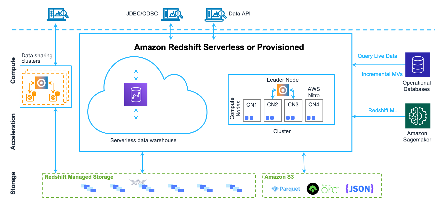
Architecture
Architecture Diagram
Redshift is composed of a cluster of one or more compute nodes. If two or more nodes are used, an additional node called Leader Node is automatically added.
Clients
Redshift can integrate with almost any SQL client via ODBC or JDBC, be it ETL tools, Business Intelligence (BI) tools, etc.
Leader Node
The leader node is the entry point to the Redshift database. Clients communicate with the Leader Node only (Compute Nodes are invisible to the clients).
Its responsabilities are:
- To parse and develop an execution plan for the requested database operations.
- To compile the code based on the execution plan, send the compiled code to the compute nodes that are storing the table referenced by the code and assign a portion of the data to each compute node.
- To aggregate the result coming from all of the compute nodes and return a response to the client.
Some SQL functions are only supported on the Leader Node.
Compute Nodes
The compute nodes are responsible for running the code given by the leader node and sending back intermediate results to the leader node for final aggregation. A compute node is partitioned into Node Slices.
Each compute node has its own dedicated CPU and memory, which are determined by the node type. It can scale on-demand (not automatically, so it is usually done during a maintenance window) both horizontally and vertically. The node types are:
- Dense Storage (DS): Focuses on storage by using HDD, which also makes it cheaper.
- Dense Compute (DC): Focuses on performance by using SSD.
- RA3: For independent scaling of compute and storage. SSD-based.
Compute nodes are set on a private network and cannot be accessed by clients directly.
Node slices
Within a compute node, there are many node slides, each of them with its own memory and disk space allocation. The leader node manages the distribution of the data/operations to the node slices, which in turn will work in parallel with other node slices to complete the requested operation.
The number of slices is dependent on the node size (type). The data can be distributed across the node slices by a column set as the distribution key, evenly in a round-robin fashion, or the entire table loaded on every nodes.
Redshift Managed Storage (RMS)
Instead of storing the data in the compute node, RMS gives the ability to store the data on S3 and provides an SSD for caching. This allows the compute nodes to be provisioned by their compute needs only.
- Hot data stored on SSD
- Cold data stored on S3
Cluster Resizing
There are two ways for adding/removing nodes to/from a cluster:
Elastic Resize
Elastic Resize is a quick method for resizing the cluster and can be used in two distinct scenarios:
- For adding or removing nodes with the same node type as the other nodes in the cluster. Some queries may be lost during the operation.
- OR for changing all the node types without changing the number of nodes. When the node type is changed, a new cluster is created, and the data is redistributed to the new cluster. Running queries are dropped when the new cluster is ready. In this scenario the cluster will be in read-only mode.
Classic Resize
A time-consuming method for when Elastic Resize cannot be used. For instance, when you need to change both node type and number of nodes. It will also create a new cluster, but will take considerably longer when compared to the Elastic Resize and the cluster will be in read-only mode.
Alternative to the Classic Resize
A workaround to avoid blocking all the write operations is to manually create a new cluster from a snapshot and then perform the classic resize in the new cluster so as not to impact the original cluster. Once the operation is completed, the delta of the data must be migrated to the new cluster.
Replication and Backup
Redshift will automatically store three copies of the data for multi-node clusters:
- Original Data
- Copy on other compute nodes inside the cluster, to be used in case of node failure.
- Copy on S3 for backup purposes.
It is possible to create automatic snapshots on S3 in another region asynchronously for disaster recovery. By default, they are stored for one day, but it can be increased to up to 35 days.
When a Redshift Cluster is terminated, all automatic generated snapshots are deleted from S3, so remember to generate a manual snapshot before termination.
To recover from a snapshot, AWS will create a new cluster in parallel with the snapshot and then make the failover to the new cluster.
Availability
In case of:
- Drive fault on a node: Cluster is still available with a slight downgrade in performance while the drive is being replaced.
- Full node fault: if single-node, Redshift becomes unavailable while the node is not replaced.
- Availability Zone fault: as Redshift is a single AZ service, it becomes unavailable while the AZ is down. One alternative is to manually restore a snapshot in another AZ.
Redshift Spectrum
Query (Read-Only) S3 unstructured data like any other table inside your Data Warehouse without affecting your Cluster, as it uses Redshift’s internal servers. It is a great tool for integrating Data Lake and Data Warehouse and separating compute and storage resources.
Provides:
- Limitless concurrency: allows the same files to be accessed simultaneously.
- Support to Parquet, Avro, JSON, and many other file formats, whether compressed (by GZIP or Snappy) or not.
- Pseudo columns $path and $size give information about the S3 files being accessed.
Data Distribution Modes
There are four modes for distributing the data across the Compute Nodes. The goal mus always be to minimize data movement across the nodes to maximize performance.
The modes are:
- AUTO: It is the default method, and it will choose the appropriate mode depending on the table size. For small tables, it starts as ALL. As the table grows, it may become EVEN. Once EVEN, it never returns to ALL.
- EVEN: the leader node distributes the data in a round-robin fashion across the Compute Nodes regardless of the data values. It is usually used when the tables do not participate in joins or when there is not a clear choice between EVEN and ALL.
- KEY: the data is distributed according to the values of a specified column. The same values go to the same node slices. Ideal for tables with a clear join key.
- ALL: the whole table is stored in every Compute Node. The storage size required is TableSize x NumberOfComputeNodes. It is ideal for short, slow-moving tables that are required for joins. Minimizes data movement but increases INSERT / UPDATE cost.
It is possible to check the distribution mode of a table by querying the PG_CLASS_INFO table.
Choosing the Distribution Mode
A general step-by-set is to:
- Specify all the Primary Keys and Foreign Keys of all tables.
- Distribute the fact table and the main dimension table by the most significant/used join key. Each table can only be distributed by a single key.
- Small and Slow-moving tables can be distributed as ALL if required by joins.
- Distribute the other tables by Primary Key or Foreign Key depending on how they are most frequently used for joins.
- Any table not used on joins or with no clear usage pattern, use EVEN distribution.
Table Constraints
- NOT NULL constraint must be respected when loading data into a Redshift Table.
Unique / Primary / Foreign Keys are not enforced by Redshift. Even still, it is a best practice to set them up so that the query optimizer can work better.
Sort Keys
Sort Keys define how the data will sorted inside of a data block on a node slice. Each data block has up to 1MB.
It works similarly to indexes in the sense that it stores the min and max values of the Sort Key as metadata on the node slice, and then when data is required for Query/Join, Redshift can simply skip whole blocks of data depending on the SQL conditions. If there is no Sort Key, the query optimizer will most likely request a full table scan.
The performance can increase for some queries if a column is set as both the Distribution Key and the Sort Key of the table, as it allows merge join to be executed instead of hash join.
New data is inserted in an “unsorted” area of the node slice, downgrading the performance. That is why it is essential to run the VACUUM command regularly.
There are three types of Sort Key:
Single Key
- A single column is the Sort Key.
Compound Sort Key
- Recommended for most tables and the default method.
- It is formed by all the columns listed in the Sort Key Columns, and the order in which they are selected is important. If only secondary columns from the Sort Key are used, the query will not fully benefit from the Sort Key.
Interleaved Sort Key
- All the Sort Key columns have the same weight, so it doesn’t matter if only “secondary” Sort Keys are used. It is more effective on huge tables as it can then skip whole blocks of 1 MB of data.
- Should not be used on columns with high cardinality (large number of unique values) such as Primary Key, Date columns, etc. On the other hand, columns with a common prefix, such as URLs (https://www.) are better on Interleaved Keys, as Compound Keys only use a small subset of the actual value.
- The downside is that it considerably increases the load and VACUUM time.
Data Ingestion
- COPY command
- Auto-copy from S3: allows data to be copied into the cluster automatically.
- Auto replication from Aurora RDBMS.
- Streaming Ingestion: from Kinesis Data Streams or Managed Streaming for Apache Kafka (MSK).
Commands
COPY
The COPY command is the recommended way for loading external data into a Redshift table, as it loads the data in a distributed fashion while also identifying the best compression algorithm per column.
The data source can be: S3, EMR, DynamoDB, and Remote Hosts (SSH). It requires a manifest file and IAM role permissions. Not possible to copy from RDS.
For narrow tables (a lot of rows but a small set of columns), it is better to load with a single transaction to reduce storage needed for metadata.
To validate the command, use the parameter NOLOAD. It is much faster because it does not write the data into the Cluster.
When data is loaded with INSERT INTO, the command is executed on the Leader Node, which is the reason for being slower.
Use Enhanced VPC Routing to force the S3 data to go through the VPC. Otherwise, the data will go through the public internet. Use Internet Gateway for services outside of the VPC or NAT Gateway for S3 buckets in other regions.
Copy from DynamoDB
- Use the READ RATIO parameter to limit the RCU used.
- The column/attribute matching is case insensitive. If there are two attibutes like ATT1 and att1, the COPY will fail.
- Attributes that do not exist in the target Redshift table are ignored.
- Columns that do not exist in the source DynamoDB table are set as Null or Empty.
- Complex data types such as SET are not supported.
Deep Copy
Deep Copy is actually a series of commands that recreates and repopulates a table by using a bulk insert, which automatically sorts the table. If a table has a large unsorted Region, a deep copy is much faster than a vacuum.
- (Optional) Recreate the table DDL by running a script called v_generate_tbl_ddl.
- Create a copy of the table using the original CREATE TABLE DDL.
- Use an INSERT INTO … SELECT statement to populate the copy with data from the original table.
- Check for permissions granted on the old table. You can see these permissions in the SVV_RELATION_PRIVILEGES system view.
- If necessary, grant the permissions of the old table to the new table.
- Grant usage permission to every group and user that has privileges in the original table. This step isn’t necessary if your deep copy table is in the public schema, or is in the same schema as the original table.
- Drop the original table.
- Use an ALTER TABLE statement to rename the copy to the original table name.
Alternatively, it is possible to:
  CREATE TABLE temp_name AS (SELECT * FROM original_table);

  TRUNCATE TABLE original_table;

  INSERT INTO original_table (SELECT * FROM temp_table);
Temporary tables are dropped when the transaction is completed and TRUNCATE table commits immediately. Therefore, there is a real risk of losing data. So use this option only when really necessary.
VACUUM
Performs re-sort of all the data and recovers storage used by deleted data. It’s also important to run ANALYZE (on the entire database, on a table, or on some columns of a table) to update the table statistics.
VACUUM DELETE ONLY only recovers the storage used by deleted records.
VACUUM SORT ONLY only reorders the data.
VACUUM REINDEX should be used when there is no Sort Key on the table or when data skewness is identified. Reinitializes Interleaved indexes. It is considerably slower then VACUUM only.
UNLOAD
Used for extracting data from Redshift into S3 in a parallel fashion. It is possible to turn off the parallelism to get a single file as output (max file size is 6.2GB). File is automatically encrypted with SSE-S3.
TRUNCATE
Deletes all the data of a table and is very fast. The TRUNCATE command commits immediately, even inside of a transaction block, which may cause data loss if used incorrectly.
GRANT or REVOKE
It is used for managing access of users and groups.
ANALYZE_COMPRESSION
It is used for analyzing the compression methods and their effectiveness per column.
Disabling session cache
By default, the cache is enabled for some frequently used queries. To disable it for the current session, run enable_result_cache_for_session=off.
CREATE EXTERNAL FUNCTION
See Lambda UDF.
BULK INSERT or Multi-row Insert
It is always preferable to use COPY. When it is not possible, however, BULK INSERT becomes the best alternative.
Materialized Views
It is possible to create materialized views in Redshift, and they can be chained - having a materialized view from another materialized view. When the underlying data changes, they must be refreshed manually or automatically if set during the materialized view creation. They are useful for improving performance of complex joins as they are already computed in the MV.
There are mainly two ways of automatically refreshing a materialized view:
- Using
AUTO REFERESH YESin theCREATEstatement: the view will refresh as soon as possible. - Using the query editor v2 to create a scheduler to refresh the view only on scheduled hours.
CREATE MATERIALIZED VIEW mv_foo
AUTO REFRESH YES --optional
AS (
  SELECT *
  FROM bar
);
System Tables/Views
- STL
- Log tables.
- STV
- Snapshot tables.
- SVV/SVL
- Views containing a subset of the STL/STV tables’ data.
- PG
- Catalogue tables.
DBLink
Extension for connecting Redshift and PostgreSQL (RDS or not).
Concurrency Scaling
Concurrency Scaling is a feature that automatically adds capacity to a new cluster to handle a burst of READ traffic. Can handle a massive number of queries and users.
Write operations are made only on the main cluster.
Read queries cannot utilize tables with interleaved sort keys or temporary ones.
Redshift Workload Management (WLM)
Query prioritization mechanism. Create queues for managing your queries, and avoid having fast queries waiting for slow queries to complete.
It can also manage which queries are sent to the concurrency scaling cluster.
WLM types are:
Automatic WLM
- Allows the creation of up to 8 queues. By default, it creates five queues with an even memory distribution between them.
- Automatically sets low concurrency for slow queries (for increased compute resources per query) and high concurrency for faster queries.
Parameters:
- Priority
- Defines the importance of the queries in the queue relative to the other queues. It is the main difference when compared to the Manual WLM.
- Concurrency Scaling
- Sets if the queue can use the concurrency scaling cluster or not.
- User Groups
- Sets which users/user groups will have their queries assigned to the queue.
- Query Groups
- Sets which query labels will be assigned to the queue. For example: Finance, Analytics, Critical, etc.
- Query monitoring rules
- Allows the query priority to change according to some pre-defined rules. Allow some actions as: change priority (for Auto WLM), log, abort and hop (for Manual WLM).
Manual WLM
Manual WLM provides, by default, one queue with a level of concurrency of five (up to 5 simultaneous queries) and a superuser queue with concurrency of one for administrative queries that must always execute. Additionally, up to 8 queues with concurrency level up to 50 can be set.
Manual WLM queues have the same parameters as Automatic queues, except the Priority one. In addition to them, there is also:
- Queue Memory
- Query timeout
- Query Queue Hopping: when a query timeouts, it will try to go to the next queue where it fits its rules to try to run again.
In manual mode, the memory of a queue is distributed evenly across all queries in execution in that queue.
Short Query Acceleration (SQA)
Prioritizes short queries by using a dedicated queue and machine learning to predict the query’s execution time. Works only with read-only queries or CREATE TABLE AS.
It is possible to set what is “short”: 1 to 20 seconds. However, the recommended is the default dynamic mode.
Redshift Serverless
A more straightforward way of creating a Redshift Cluster is using the Serverless Mode. It provides auto-scaling, auto-provisioning, good performance backed up by Machine Learning algorithms, and pay only when in use billing. Data is encrypted by KMS by default. Additionally, there is no WLM concept, as this is done automatically via Machine Learning.
The main drawbacks are that Redshift Spectrum and Maintenance Windows are currently not supported by Redshift Serverless. Additionally, there is no public DNS available. The access must be done from inside of a VPC.
Cost
While Redshift Cluster is billed by the number and type of nodes provisioned, the serverless mode is billed by Redshift Processing Units (RPU) plus storage.
By default, the RPU mode is set to AUTO. However, it is possible to set a range so that at least a minimum RPU is always available and the RPU usage does not exceed a maximum value.
Redshift DataLake Export
Enables us to unload Redshift data to S3 in a partitioned Parquet file.
UDFs and Stored Procedures
Redshift UDF
Supports SQL or Python.
Lambda UDF
It is possible to use a Lambda function (same account or cross-account but same region) as a UDF SQL Function. Redshift and Lambda will communicate using JSON. The only requirement is to GRANT USAGE ON LANGUAGE EXFUNC.
For registering a Lambda UDF:
CREATE EXTERNAL FUNCTION function_name(param1_type, paramN_type)
RETURNS return_type VOLATILE LAMBDA 'lambda_name'
IAM_ROLE 'arn:aws:iam:...';
Stored Procedures
Similar to UDF, but are defined using PL/pgSQL (PostgreSQL Procedural Language) and are able to execute DDL and DML operations.
Federated Queries
Federated Queries is a simple way of querying external data (read-only) from relational databases (RDS), data warehouses (another Redshift cluster), and lakes (S3). Credentials must be stored in the AWS Secrets Manager, the Redshift cluster must have access to the Credentials via IAM Role permission, and services must be on the same VPC; otherwise, VPC peering must be used.
- CREATE EXTERNAL SCHEMA is used for creating a Federated Query connection.
- It is possible to see all available Federated Queries by querying SVV_EXTERNAL_SCHEMAS.
Data Sharing
It is possible to share live read-only data in a secure manner, cross-region (incur extra charges), or even cross-account with other Redshift clusters without the need to copy data. The only requirement is to have RA3 node type, and both nodes must be encrypted.
Advanced Query Accelerator (AQUA)
A distributed and hardware-accelerated cache at no extra cost. Requires RA3 node type.
Hardware Security Module (HSM)
- A client and server certificate must be used to connect the HSM module and the Redshift Cluster.
- There is no way of directly creating an HSM-encrypted cluster from a snapshot of a non HSM-encrypted cluster. To do that, one must first create an HSM-encrypted cluster and then migrate (copy) the data from a non-encrypted one.
Redshift Advisor
Gives recommendations on performance improvement and cost reduction.